HBP Handgrip Report

Grip Strength Patterns Across Athletic and Population Cohorts

Exploratory frequentist analysis comparing dominant-hand grip strength across SG25 athletes, NHANES exercisers, and NHANES non-exercisers, with within-group contrasts by self-reported high blood pressure (HBP).

Code

getwd()

[1] "/Users/leej/Documents/codex-managed/projects/research-hub/analysis"

Prepare Cohorts

Code

library(dplyr)
library(tidyr)

prepared <- combined %>%
  mutate(
    meets_guidelines = case_when(
      meets_ACSM_guidelines %in% c(TRUE, 1, "Yes", "Y") ~ TRUE,
      meets_ACSM_guidelines %in% c(FALSE, 0, "No", "N") ~ FALSE,
      TRUE ~ NA
    ),
    activity_group = case_when(
      dataset == "SG25" ~ "SG_Athletes",
      dataset == "NHANES" & meets_guidelines %in% TRUE ~ "NHANES_Exercisers",
      dataset == "NHANES" & meets_guidelines %in% FALSE ~ "NHANES_NonExercisers",
      TRUE ~ NA_character_
    ),
    hbp_status = if_else(HBP %in% c(TRUE, 1, "Yes", "Y"), "HBP_Yes", "HBP_No")
  ) %>%
  filter(!is.na(activity_group), is.finite(grip_dom))

cohorts <- prepared

dplyr::count(cohorts, activity_group, hbp_status)

# A tibble: 6 × 3
  activity_group       hbp_status     n
  <chr>                <chr>      <int>
1 NHANES_Exercisers    HBP_No      1136
2 NHANES_Exercisers    HBP_Yes     1101
3 NHANES_NonExercisers HBP_No       835
4 NHANES_NonExercisers HBP_Yes     1286
5 SG_Athletes          HBP_No        78
6 SG_Athletes          HBP_Yes       37

Grip Strength Summary Tables

Code

library(gt)
group_levels <- c("SG_Athletes", "NHANES_Exercisers", "NHANES_NonExercisers")

grip_summary_overall <- cohorts %>%
  mutate(activity_group = factor(activity_group, levels = group_levels)) %>%
  group_by(activity_group) %>%
  summarise(
    n = n(),
    mean_grip = mean(grip_dom, na.rm = TRUE),
    sd_grip = sd(grip_dom, na.rm = TRUE),
    .groups = "drop"
  ) %>%
  mutate(summary = sprintf("%.2f ± %.2f (n=%d)", mean_grip, sd_grip, n))

grip_summary_overall

# A tibble: 3 × 5
  activity_group           n mean_grip sd_grip summary               
  <fct>                <int>     <dbl>   <dbl> <chr>                 
1 SG_Athletes            115      38.9    11.7 38.89 ± 11.74 (n=115) 
2 NHANES_Exercisers     2237      35.1    10.5 35.07 ± 10.48 (n=2237)
3 NHANES_NonExercisers  2121      30.7    10.3 30.73 ± 10.31 (n=2121)

Code

gt_overall <- grip_summary_overall %>%
  gt() %>%
  tab_header(
    title = "Dominant-Hand Grip Strength by Activity Group",
    subtitle = "Mean ± SD (n) across SG athletes and NHANES exerciser/non-exerciser cohorts"
  )

gt_overall

activity_group	n	mean_grip	sd_grip	summary
Dominant-Hand Grip Strength by Activity Group
Mean ± SD (n) across SG athletes and NHANES exerciser/non-exerciser cohorts
SG_Athletes	115	38.88870	11.74300	38.89 ± 11.74 (n=115)
NHANES_Exercisers	2237	35.06737	10.48217	35.07 ± 10.48 (n=2237)
NHANES_NonExercisers	2121	30.73442	10.31196	30.73 ± 10.31 (n=2121)

Code

grip_summary_within <- cohorts %>%
  filter(!is.na(hbp_status)) %>%
  mutate(activity_group = factor(activity_group, levels = group_levels)) %>%
  group_by(activity_group, hbp_status) %>%
  summarise(
    n = n(),
    mean_grip = mean(grip_dom, na.rm = TRUE),
    sd_grip = sd(grip_dom, na.rm = TRUE),
    .groups = "drop"
  ) %>%
  mutate(
    summary = sprintf("%.2f ± %.2f (n=%d)", mean_grip, sd_grip, n)
  ) %>%
  select(activity_group, hbp_status, summary) %>%
  pivot_wider(
    names_from = hbp_status,
    values_from = summary,
    values_fill = "—"
  ) %>%
  arrange(activity_group)

grip_summary_within

# A tibble: 3 × 3
  activity_group       HBP_No                 HBP_Yes               
  <fct>                <chr>                  <chr>                 
1 SG_Athletes          39.07 ± 11.78 (n=78)   38.51 ± 11.81 (n=37)  
2 NHANES_Exercisers    35.28 ± 10.30 (n=1136) 34.85 ± 10.66 (n=1101)
3 NHANES_NonExercisers 31.86 ± 10.03 (n=835)  30.00 ± 10.43 (n=1286)

Code

gt_within <- grip_summary_within %>%
  gt() %>%
  tab_header(
    title = "Dominant-Hand Grip Strength by Activity Group and HBP Status",
    subtitle = "Mean ± SD (n) stratified by hypertension history"
  )

gt_within

activity_group	HBP_No	HBP_Yes
Dominant-Hand Grip Strength by Activity Group and HBP Status
Mean ± SD (n) stratified by hypertension history
SG_Athletes	39.07 ± 11.78 (n=78)	38.51 ± 11.81 (n=37)
NHANES_Exercisers	35.28 ± 10.30 (n=1136)	34.85 ± 10.66 (n=1101)
NHANES_NonExercisers	31.86 ± 10.03 (n=835)	30.00 ± 10.43 (n=1286)

Frequentist Comparisons

Code

library(broom)
library(purrr)

ttest_within_results <- cohorts %>%
  filter(!is.na(hbp_status)) %>%
  group_by(activity_group) %>%
  summarise(
    test = list(
      if (n_distinct(hbp_status) == 2) {
        tidy(t.test(grip_dom ~ hbp_status, conf.level = 0.95))
      } else {
        tibble(
          estimate = NA_real_,
          statistic = NA_real_,
          p.value = NA_real_,
          conf.low = NA_real_,
          conf.high = NA_real_
        )
      }
    ),
    .groups = "drop"
  ) %>%
  tidyr::unnest(test) %>%
  mutate(activity_group = factor(activity_group, levels = group_levels))

ttest_within_results

# A tibble: 3 × 11
  activity_group       estimate estimate1 estimate2 statistic  p.value parameter
  <fct>                   <dbl>     <dbl>     <dbl>     <dbl>    <dbl>     <dbl>
1 NHANES_Exercisers       0.424      35.3      34.9     0.955  3.40e-1    2225. 
2 NHANES_NonExercisers    1.86       31.9      30.0     4.11   4.21e-5    1831. 
3 SG_Athletes             0.557      39.1      38.5     0.237  8.14e-1      70.7
# ℹ 4 more variables: conf.low <dbl>, conf.high <dbl>, method <chr>,
#   alternative <chr>

Code

model_ready <- cohorts %>%
  mutate(
    activity_group = factor(activity_group, levels = group_levels),
    hbp_status = factor(hbp_status, levels = c("HBP_No", "HBP_Yes"))
  )

anova_overall <- broom::tidy(aov(grip_dom ~ activity_group, data = model_ready))

anova_overall

# A tibble: 2 × 6
  term              df   sumsq meansq statistic   p.value
  <chr>          <dbl>   <dbl>  <dbl>     <dbl>     <dbl>
1 activity_group     2  24380. 12190.      112.  3.70e-48
2 Residuals       4470 486836.   109.       NA  NA

Code

anova_by_hbp <- model_ready %>%
  filter(!is.na(hbp_status)) %>%
  group_by(hbp_status) %>%
  nest() %>%
  mutate(
    tidy = map(data, ~ broom::tidy(aov(grip_dom ~ activity_group, data = .x)))
  ) %>%
  select(hbp_status, tidy) %>%
  tidyr::unnest(tidy)

anova_by_hbp

# A tibble: 4 × 7
# Groups:   hbp_status [2]
  hbp_status term              df   sumsq meansq statistic   p.value
  <fct>      <chr>          <dbl>   <dbl>  <dbl>     <dbl>     <dbl>
1 HBP_Yes    activity_group     2  15384.  7692.      69.0  7.31e-30
2 HBP_Yes    Residuals       2421 269952.   112.      NA   NA       
3 HBP_No     activity_group     2   7669.  3835.      36.5  2.69e-16
4 HBP_No     Residuals       2046 215026.   105.      NA   NA

Code

lm_results <- broom::tidy(
  lm(
    grip_dom ~ activity_group + hbp_status + activity_group:hbp_status,
    data = model_ready
  )
) %>%
  mutate(across(where(is.numeric), round, digits = 4))

lm_results

# A tibble: 6 × 5
  term                                      estimate std.error statistic p.value
  <chr>                                        <dbl>     <dbl>     <dbl>   <dbl>
1 (Intercept)                                 39.1        1.18   33.1     0     
2 activity_groupNHANES_Exercisers             -3.79       1.22   -3.11    0.0019
3 activity_groupNHANES_NonExercisers          -7.21       1.23   -5.84    0     
4 hbp_statusHBP_Yes                           -0.557      2.08   -0.268   0.789 
5 activity_groupNHANES_Exercisers:hbp_stat…    0.134      2.13    0.0628  0.950 
6 activity_groupNHANES_NonExercisers:hbp_s…   -1.30       2.13   -0.611   0.541

Visualize Grip Distributions

Code

library(ggplot2)

grip_plot <- cohorts %>%
  filter(!is.na(hbp_status)) %>%
  mutate(
    activity_group = factor(activity_group, levels = group_levels),
    hbp_status = factor(hbp_status, levels = c("HBP_No", "HBP_Yes"))
  ) %>%
  ggplot(aes(x = activity_group, y = grip_dom, fill = hbp_status)) +
  geom_violin(alpha = 0.4, trim = FALSE) +
  geom_boxplot(width = 0.12, position = position_dodge(width = 0.9), outlier.shape = NA) +
  stat_summary(fun = mean, geom = "point", shape = 21, size = 2.5, position = position_dodge(width = 0.9)) +
  scale_fill_manual(values = c("HBP_No" = "#1b9e77", "HBP_Yes" = "#d95f02")) +
  labs(
    title = "Grip Strength Distributions by Activity Group and HBP History",
    x = NULL,
    y = "Dominant-hand grip (kg)",
    fill = "HBP Status"
  ) +
  theme_minimal()

grip_plot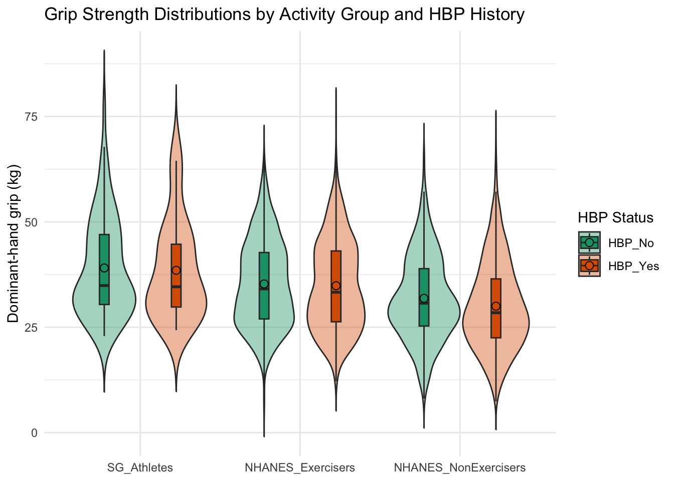

Persist Artifacts

Code

table_path <- here::here("analysis", "artifacts", "tables", "hbp-grip-summary.rds")
figure_path <- here::here("analysis", "artifacts", "figures", "hbp-grip-boxplot.png")

dir.create(dirname(table_path), showWarnings = FALSE, recursive = TRUE)
dir.create(dirname(figure_path), showWarnings = FALSE, recursive = TRUE)

saveRDS(
  list(
    overall = grip_summary_overall,
    by_hbp = grip_summary_within
  ),
  table_path
)
ggsave(figure_path, plot = grip_plot, width = 8, height = 5, dpi = 300)

list(table_rds = table_path, figure_png = figure_path)

$table_rds
[1] "/Users/leej/Documents/codex-managed/projects/research-hub/analysis/artifacts/tables/hbp-grip-summary.rds"

$figure_png
[1] "/Users/leej/Documents/codex-managed/projects/research-hub/analysis/artifacts/figures/hbp-grip-boxplot.png"

Next Steps

Extend the frequentist framework with adjusted models (e.g., age, sex, BMI covariates) if confounders are suspected.
Re-run the analysis after refreshing combined_NHANES_SG25_activity_harmonized.rds to capture updated cohorts.
Use these artifacts in downstream manuscripts or summaries by referencing the paths recorded in the document metadata.

Prepare Cohorts

Grip Strength Summary Tables

Frequentist Comparisons

Visualize Grip Distributions

Persist Artifacts

Next Steps

References